Image Feature Extraction: Local Binary Patterns with Cython
Introduction
The common goal of feature extraction is to represent the raw data as a reduced set of features that better describe their main features and attributes [1]. This way, we can reduce the dimensionality of the original input and use the new features as an input to train pattern recognition and classification techniques.
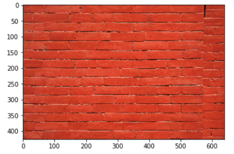
Although there are several features that we can extract from a picture, Local Binary Patterns (LBP) is a theoretically simple, yet efficient approach to grayscale and rotation invariant texture classification. They work because the most frequent patterns correspond to primitive microfeatures such as edges, corners, spots, flat regions [2].
In [2], Ojala et al. showed that the discrete occurrence histogram of the uniform patterns is a very powerful texture feature. Image texture is defined as a two-dimensional phenomenon characterized by two properties: (1) spatial structure (pattern) and (2) contrast.
Methodology
Circularly Symmetric Neighbor Set

A circularly symmetric neighbor set for a given pixel gc is defined by the points with coordinates (i, j) that surround the central point on a circle of radius R, and a number of elements P.

Texture
We define a texture T as the collection of pixels in a gray-scale image

where gp corresponds to the gray value of the p local neighbor.
Interpolation
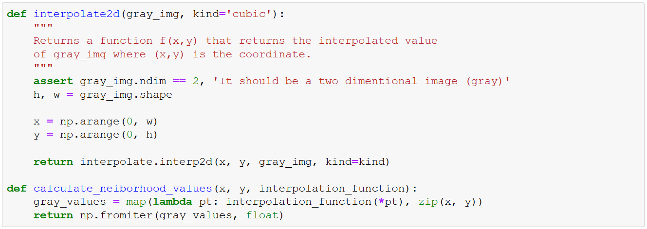
When a neighbor is not located in the center of a pixel, that neighbor gray value should be calculated by interpolation. Thus, we need to define a function that given a coordinate, returns the interpolated gray value.
Achieving Gray-Scale Invariance
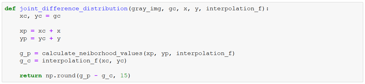
Considering a possible loss of information, it is possible to turn the texture into the joint difference. To calculate it, we subtract the gray value of the central pixel to all of the neighbor set. The joint difference distribution is a highly discriminative texture operator. It records the occurrences of various patterns in the neighborhood of each pixel in a P-dimensional histogram.

where gp is the gray value of the p neighbor. This distribution is invariant against gray-scale shifts.

Local Binary Pattern
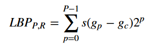
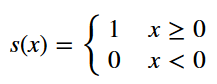
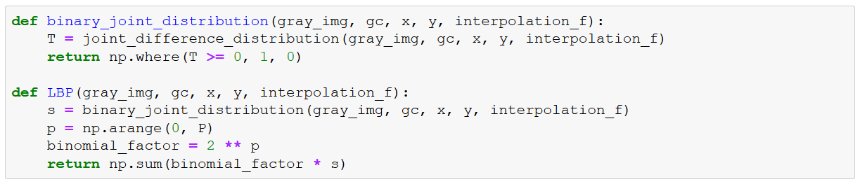
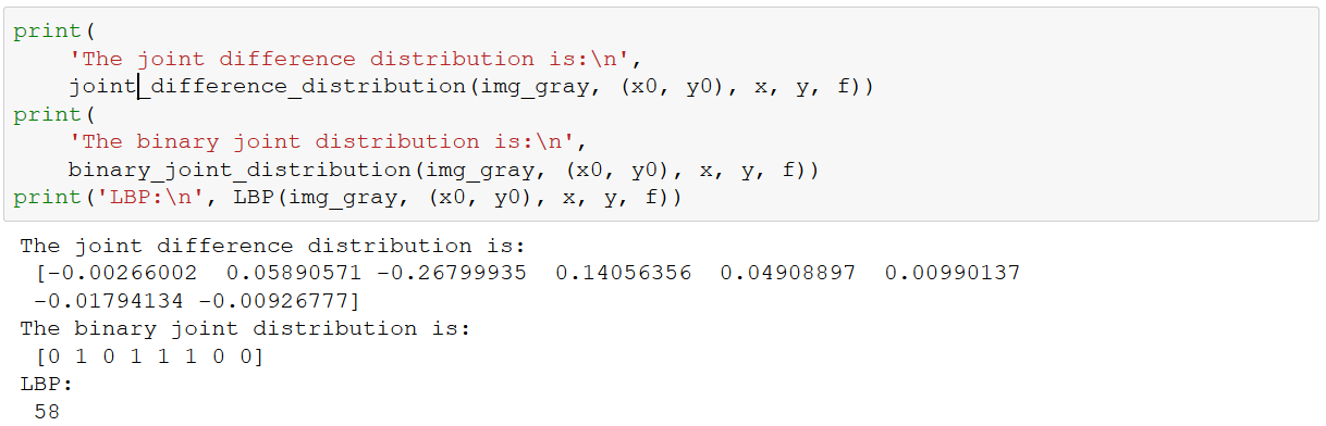
LBP_{P,R} operator is by definition invariant against any monotonic transformation of the gray-scale. As long as the order of the gray values stays the same, the output of the LBP_{P,R} operator remains constant.
where
Uniform Local Binary Patterns
In [2], Ojala mentions that in their practical experience LBP is not a good discriminator. They propose just to select the set of local binary patterns such that the number of spatial transitions (bitwise 0/1 changes) does not exceed 2. For example, the pattern ‘1111’ has 0 spatial transitions, the pattern ‘1100’ has 1 spatial transitions and the pattern ‘1101’ has 2 spatial transitions. To each uniform pattern, a unique index is associated. The formula to create the index was borrowed from here.
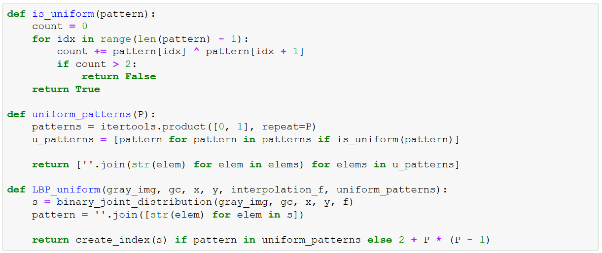
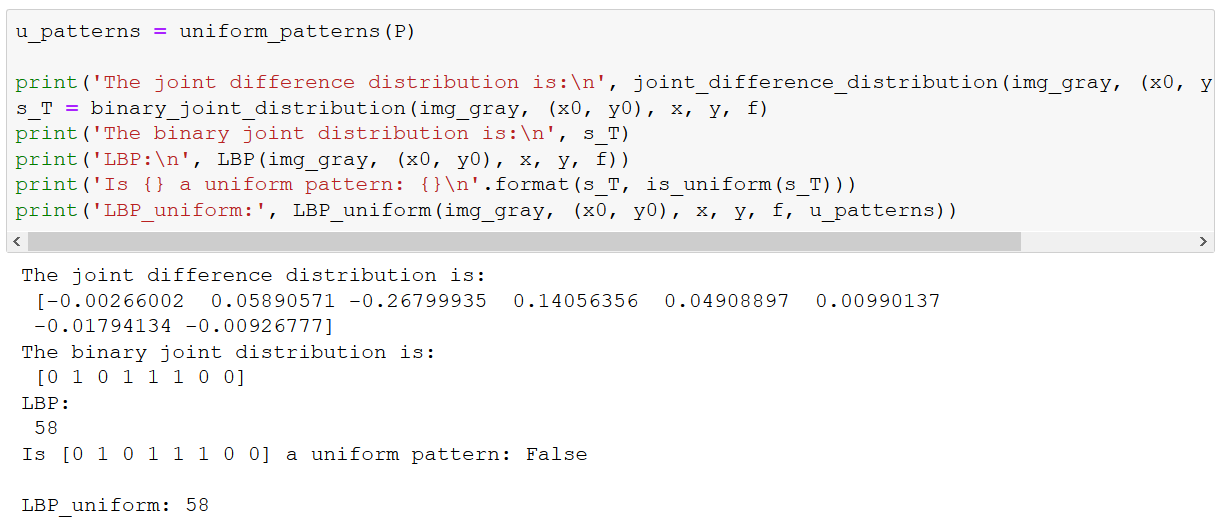
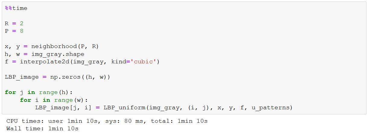
Now, we can calculate the local binary patterns for a central pixel. The next step is to calculate the local binary patterns for all the pixels.
Hint: For simplicity sake, I am not considering the case where a selected index is negative (i.e. img_gray[-1][0] returns the last pixel of the first column). If we would want to have a more accurate calculation, we should consider this case and treat it.
Cython Code
The previous code is not perfect; however, what makes it really slow is that we iterate through all the image pixels. Waiting 1 minute and 10 seconds to calculate our features is a lot if we take into account that we have also to train a pattern recognition technique. Thus, we need an alternative implementation that must be much faster for loops. In this case, we will use Cython. The code is presented in the next image, it is a big chunk of code. Some parts of it could be improved, but it is already much faster. Please feel free to leave comments if you don’t understand something from the code.
The code is written in such a way that most of it runs entirely in the C API. This strategy speeds up the execution considerably, but also allow us to take advantage of Cython’s parallel module. We will split the job across multiple cores in the CPU.
from libc.math cimport sin, cos, pi, ceil, floor, pow
from libc.stdlib cimport abort, malloc, free
import numpy as np
cimport numpy as np
cimport cython
from cython.parallel import prange, parallel
cimport openmp


cdef double get_pixel2d(
    double *image,
    Py_ssize_t n_rows,
    Py_ssize_t n_cols,
    long x,
    long y) nogil:

    if (y < 0) or (y >= n_rows) or (x < 0) or (x >= n_cols):
        return 0
    else:
        return image[y * n_cols + x]


cdef double bilinear_interpolation(
    double *image,
    Py_ssize_t n_rows,
    Py_ssize_t n_cols,
    double x,
    double y) nogil:

    cdef double d_y, d_x, top_left, top_right, bottom_left, bottom_right
    cdef long min_y, min_x, max_y, max_x

    min_y = <long>floor(y)
    min_x = <long>floor(x)
    max_y = <long>ceil(y)
    max_x = <long>ceil(x)

    d_y = y - min_y
    d_x = x - min_x

    top_left = get_pixel2d(image, n_rows, n_cols, min_x, min_y)
    top_right = get_pixel2d(image, n_rows, n_cols, max_x, min_y)
    bottom_left = get_pixel2d(image, n_rows, n_cols, min_x, max_y)
    bottom_right = get_pixel2d(image, n_rows, n_cols, max_x, max_y)

    top = (1 - d_x) * top_left + d_x * top_right
    bottom = (1 - d_x) * bottom_left + d_x * bottom_right

    return (1 - d_y) * top + d_y * bottom


cdef double *joint_difference_distribution(
    double *image,
    Py_ssize_t n_rows,
    Py_ssize_t n_cols,
    int x0,
    int y0,
    int P,
    int R
) nogil:
    cdef Py_ssize_t p
    cdef double *T = <double *> malloc(sizeof(double) * P)
    cdef double x, y, gp, gc

    if T is NULL:
        abort()

    gc = get_pixel2d(image, n_rows, n_cols, x0, y0)

    for p in range(P):
        x = x0 + R * cos(2 * pi * p / P)
        y = y0 - R * sin(2 * pi * p / P)
        gp = bilinear_interpolation(image, n_rows, n_cols, x, y)
        T[p] = gp - gc

    return T


cdef int *binary_joint_distribution(double *T, Py_ssize_t T_size) nogil:
    cdef int *s_T = <int *> malloc(sizeof(int) * T_size)
    cdef Py_ssize_t i = 0

    for t in range(T_size):
        if T[t] >= 0.0:
            s_T[t] = 1
        else:
            s_T[t] = 0

    return s_T


cdef long LBP(double *T, int *s_T, Py_ssize_t T_size) nogil:
    cdef long LBP_pr = 0
    cdef Py_ssize_t i = 0

    for i in range(0, T_size):
        LBP_pr = LBP_pr + 2 ** i * s_T[i]

    return LBP_pr


cdef int is_uniform_pattern(int *s_T, Py_ssize_t s_T_size) nogil:
    cdef Py_ssize_t i = 0
    cdef int counter = 0

    for i in range(s_T_size - 1):
        if s_T[i] != s_T[i + 1]:
            counter += 1

        if counter > 2:
            return 0
    return 1


cdef int create_index(int *s_T, Py_ssize_t s_T_size) nogil:
    cdef int n_ones = 0
    cdef int rot_index = -1
    cdef int first_one = -1
    cdef int first_zero = -1
    cdef int lbp = -1

    cdef Py_ssize_t i
    for i in range(s_T_size):
        if s_T[i]:
            n_ones += 1
            if first_one == -1:
                first_one = i
        else:
            if first_zero == -1:
                first_zero = i

    if n_ones == 0:
        lbp = 0
    elif n_ones == s_T_size:
        lbp = s_T_size * (s_T_size - 1) + 1
    else:
        if first_one == 0:
            rot_index = n_ones - first_zero
        else:
            rot_index = s_T_size - first_one
        lbp = 1 + (n_ones - 1) * s_T_size + rot_index
    return lbp


cdef int LBP_uniform(int *s_T, Py_ssize_t s_T_size) nogil:
    cdef int LBP_pru = 0
    cdef Py_ssize_t i = 0

    if is_uniform_pattern(s_T, s_T_size):
        LBP_pru = create_index(s_T, s_T_size)
    else:
        LBP_pru = 2 + s_T_size * (s_T_size - 1)

    return LBP_pru


@cython.boundscheck(False)
@cython.wraparound(False)
def local_binary_patterns(
    double[:, ::1] image,
    int P,
    int R,
    int num_threads=1
):

    cdef Py_ssize_t x = 0
    cdef Py_ssize_t y = 0
    cdef int n_rows = image.shape[0]
    cdef int n_cols = image.shape[1]
    cdef int[:, ::1] lbp = np.zeros([n_rows, n_cols], dtype=np.int32)

    with nogil, parallel(num_threads=num_threads):
        for y in prange(n_rows, schedule='static'):
            for x in prange(n_cols, schedule='static'):
                T = joint_difference_distribution(&image[0][0], n_rows, n_cols, x, y, P, R)
                s_T = binary_joint_distribution(T, P)
                lbp[y, x] = LBP_uniform(s_T, P)

    return np.asarray(lbp)
Using 4 threads, we could calculate the local binary patterns for all the pixels in less than 150 ms. This is so much faster that I won’t even bother to calculate by how many times.

Comparison with a Similar Image
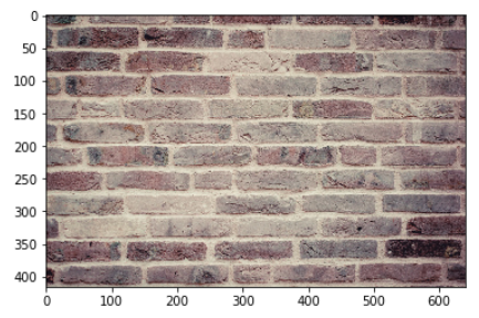
Let’s take another image of bricks, but this one will have a different texture.
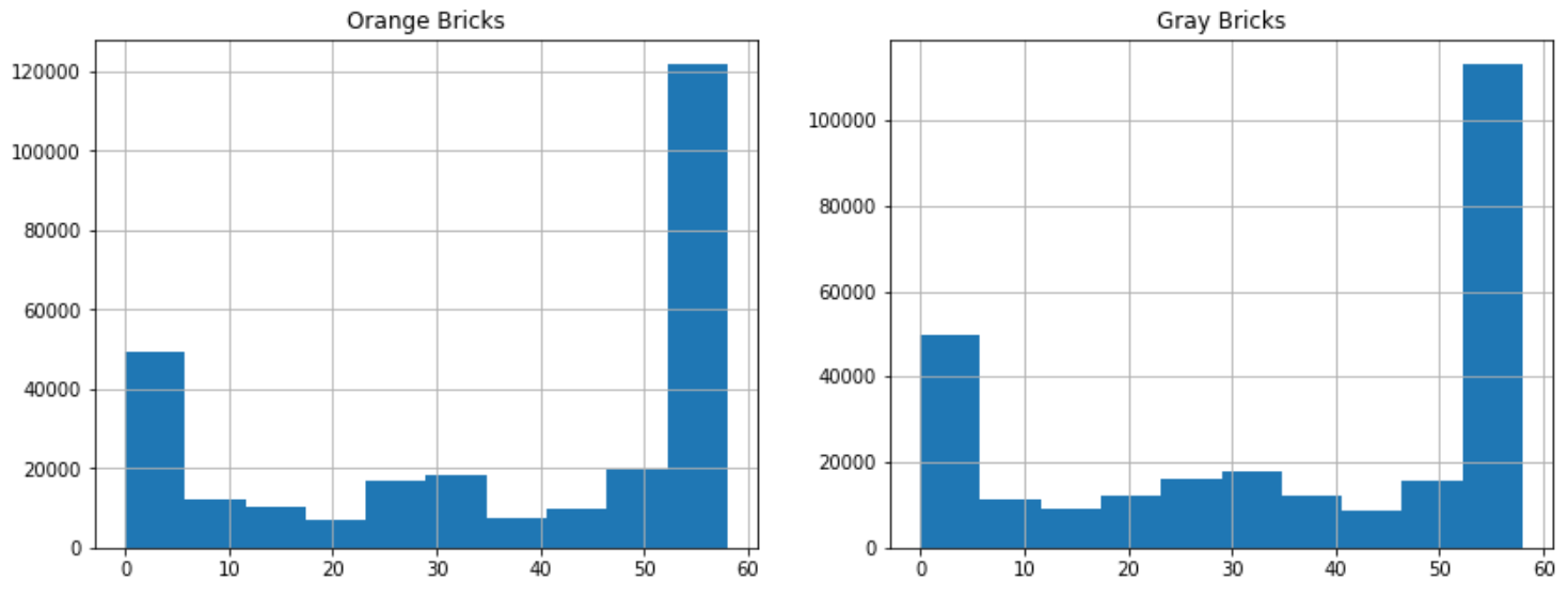
Both histograms are very similar, and they should be, in the end both of them are bricks. Nonetheless, features from 20 to 40 are very dissimilar in both images. It means that with a good machine learning algorithm we could correctly classify them.
Conclusion
Local binary patterns are simple but efficient features. The theory behind is not hard to understand and they are easy to code. Nevertheless, if we code them entirely with Python, we will have some performance issues. We tackled the problem with Cython and we got very impressive results. The next step is to collect different texture images and train your favorite machine learning algorithm to classify them.
Jupyter Notebook
Bibliography
[1] Marques, O. (2011). Practical image and video processing using MATLAB. John Wiley & Sons.
[2] Ojala, T., Pietikäinen, M., & Mäenpää, T. (2002). Multiresolution gray-scale and rotation invariant texture classification with local binary patterns. IEEE Transactions on Pattern Analysis and Machine Intelligence, 24(7), 971–987.
Image Feature Extraction: Local Binary Patterns with Cython was originally published in HackerNoon.com on Medium, where people are continuing the conversation by highlighting and responding to this story.